Investment risk and return analysis using VeriPlan’s Excel Monte Carlo analysis features

VeriPlan’s Excel Monte Carlo analysis features simplify investment risk and return analysis

To simplify investment risk and return analysis, VeriPlan’s “Painless” Excel Monte Carlo investment performance variation method allows you to project investment performance with parameters that systematically vary compounded historical real dollar returns with inflation removed that are below or above VeriPlan’s 50th percentile centerline projections. This Monte Carlo Variance Tool is based upon our systematic Monte Carlo statistical sampling study of US historical bond and stock returns.

Using almost 100 years of US data, the Monte Carlo statistical sampling method was used to simulate investment portfolio performance across 11 bond and stock asset allocations, 3 investment models, and 6 different decade-long time periods. By sampling each of these 198 combinations 5,000,000 times, the range of terminal portfolio values was calculated, rank ordered by percentile, and embedded into VeriPlan’s core investment projection logic.

Overview of Excel Monte Carlo Analysis features in VeriPlan’s Portfolio Risk worksheet

1) VeriPlan’s investment risk & return methods to vary investment asset class return assumptions and values

VeriPlan provides four facilities to simulate investment projection variability. These methods develop projections for the cash, bond, and stock financial asset classes. Some of these methods allow you to develop projections with return assumptions that differ from VeriPlan’s 50 percentile, “centerline” assumptions, which are detailed on the adjacent Portfolio Return worksheet. While these methods are automatically combinable, you are encouraged to use them one at a time, so that you will have a more clear understanding of how to interpret these altered projections.

• The Monte Carlo Variance Tool allows you to vary bond and stock asset class returns by individual percentiles from 1% to 99% with the 50th percentile equaling VeriPlan’s centerline projection assumptions.
• The Standard Deviation Variance Tool allows you to vary financial asset class returns in proportion to their historical volatility or risk.
• The Current Portfolio Revaluation Tool adjusts your current financial assets simulate substantial near-term asset value changes without any long-term recovery.
• The Safety Margin Tool projects how long your cash and bonds would pay the bills without other income or stock assets.

If you wish to change the real dollar financial asset class growth rates that are used by VeriPlan upward or downward, use Methods A or B. The natural human tendency is to test the negative or downside, but since the future is not predictable, whenever you test for a downside metric, you should also test for the corresponding upside metric to develop an appreciation for the uncertainty of the future and the risks and benefits of owning financial investment assets.

Some VeriPlan users might wish to understand how substantial near-term changes to the value of their current portfolio might affect their lifetime projections. The current portfolio revaluation tool provides an efficient means to revalue your current portfolio, so that your projection baseline will start with lower or higher asset class values. Nevertheless, you should be careful in assuming that asset valuation markets are “wrong” and that such current “wrong” valuations will be sustained into the future. At any point in time, it is difficult to evaluate whether current markets are over- or under-valuing assets with respect to the long-term.

2) Setting VeriPlan’s Excel Monte Carlo variance analysis tool

VeriPlan’s Monte Carlo Variance Tool is a investment performance variance facility based on the Monte Carlo statistical method. It allows you to project investment performance using parameters that systematically vary your financial investment returns below or above the compounded returns of the 50th percentile centerline projection.

With this tool, the user can enter any whole integer number from 1 to 99 to select long-term historical real dollar bond and stock performance percentiles that are ordered from the least (number 1) to the greatest (number 99), using the almost of 100 year historical performance record. The 50 percentile equals VeriPlan’s centerline investment parameters. For any percentile you choose, VeriPlan’s projections will automatically take into account your particular strategic bond to stock asset allocation, when it varies your investment performance parameters.

VeriPlan’s Monte Carlo Variance Tool is based upon a systematic Monte Carlo statistical sampling study of historical bond and stock real dollar returns that used various asset allocations, investment models, and investment holding periods. Using almost 100 years of data, the Monte Carlo statistical sampling method was used to simulate investment portfolio performance across 11 asset allocations, 3 investment models, and 6 different decade-long time periods. By sampling these 198 combinations 5,000,000 times each, the range of portfolio value outcomes was calculated for each of the combinations.

For more details, lower on this worksheet you will find a section titled “Explanation of the Monte Carlo Variance Tool.”

VeriPlan’s approach to Monte Carlo simulation does not interfere with a user’s development of their lifetime financial projection models. If a user decides to vary their investment return assumptions using VeriPlan’s Monte Carlo percentile mechanism, changes to their projections will still be characterized by sub-second computer response time.

How to use VeriPlan’s Monte Carlo Variance Tool

Depending up the whole number integer, between 1 and 99, that you enter in the gray box below, VeriPlan will develop projections representing historical performance percentile outcomes ordered from the least (1) to greatest (99).

To use this investment portfolio variation tool simply choose an historical bond and stock performance percentile:

• Enter any whole integer from 1 to 99 (The default “centerline” percentile is 50)
• The resulting bond and stock return variance multiplication factor will be shown

While the natural tendency is to choose performance outcomes below the 50th percentile, it is important that you evaluate projections that are the mirror image of your skepticism. If you evaluate the 25th percentile, also evaluate the 75th percentile, etc.

Develop perspective on the interpretation of your portfolio’s investment risk and return performance variance

If you intend to use this Monte Carlo Variance Tool, you should study the section below titled “Explanation of the Monte Carlo Variance Tool.” In particular, look across the 1 to 99 percentile charts, while noting the particular bond and stock asset allocation lines that are closest to your chosen asset allocation on the yellow-tabbed Asset Allocation worksheet.

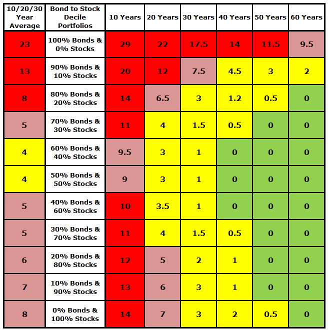
The table below is pessimistic perspective analysis focused on real dollar investment losses. A similar analysis could have be performed relative to any arbitrary positive cumulative performance outcome, such as 2%, 5%, etc., but losses are what people tend to fear most. This is an analysis of the total number of loss percentiles, across all 11 asset allocations, 3 investment models, and 6 different decade-long time periods. A cumulative loss percentile is one in which the Internal Rate of Return was negative in real, constant purchasing power dollar terms. This means that the dollars invested initially and through the years ended up being worth less at the end of the period than their invested values. The user’s particular asset allocation and holding period made a significant difference in these loss percentile outcomes. The three investment models did not.

Clearly, in these extensive simulations, a more balanced and diversified portfolio with to both bonds and stocks experienced fewer loss years than either bond heavy or stock heavy asset allocations. One might be surprised that 100% bond portfolios experienced many more loss years than 100% stock portfolios. You should note that this Monte Carlo study was conducted using the 10-Year US Treasury bond performance history from 1928 to 2023. Instead of repetition here, you are encouraged to read Section 1 of the adjacent yellow-tabbed Portfolio Return worksheet titled: “Apportion your projected bond returns between US Treasury and AAA bonds.” While very safe and a proxy for the long-term risk free rate of return, Treasury bonds have had about a 1.5% compounded return in real dollars over the years. Whereas stocks, as measured by the S & P Index, have experienced a compounded return of about 6.75% in excess of inflation over the same period.

The number of decades for the investment period also made a significant difference, however, the 40, 50, and 60 year periods were quite similar for all but the very bond heavy asset allocations. The decision was made to average the 10, 20, and 30 year periods, since this is a long-term / lifelong financial planning application. This 10, 20, and 30 year average will understate the variation of the 10 year holding period and overstate the variation of holding periods longer than 20 years. Given the complexity of this simulation modeling exercise it was decided not to incorporate each decade into the model. If you are spending a lot of time modeling your lifetime projection with very pessimistic assumptions, you can make mental adjustments by some number of percentiles, if your time frame is short or longer. However, you should ask yourself why your focus is shorter-term, unless you are quite old already.

Regarding investment models, they made no material difference in this Monte Carlo study. Each of the three investment models invested $1,000 initially. Then, each model invested either $0, $100, or $200 each year thereafter across the number of years under consideration for each decade-long period. For example, one would expect to see the greatest difference between the was there a single percentile difference. The other 52 out of 66 table entries were the same. You can detect those that had a difference in the chart below whenever and entry ends in “x.5”, which is the average of the $1,000/+$0 and $1,000/+$100 investment models.

Number of US long-term return percentiles out of the 99 with cumulative losses conditioned by decile stock and bond strategic asset allocations

VeriPlan’s Excel Monte Carlo analysis explained

Overview of the Monte Carlo statistical method

In probability and statistics, the “normal,” bell-shaped statistical distribution model is used most often, because it is a reasonable method to model variation within many population distributions. However, historical investment data tends to be characterized by significantly more negative and positive outcomes than the normal, bell-shaped distribution would predict. Thus, historical investment data creates a “fat-tails” problem for the normal distribution.

The Monte Carlo method can overcome these statistical problems. If you desire more detailed background information, just search ” Monte Carlo method ” in your favorite browser.

In summary, the Monte Carlo method requires: a) an input data set, b) a randomized sampling method, and c) a sampling engine. When the sampling engine runs a large number of random samples against the input data set, a probability distribution that characterizes the data will emerge. When a sufficiently large number of samples are drawn, the statistical “law of large numbers” indicates that the sample distribution should approximate the actual distribution of the data.

There are several problems with how the Monte Carlo method often has been applied to investment performance projections, including:

• limited historical periods, when much longer data series are available,
• ignoring correlations between asset classes,
• the cumbersomeness of calculations, and
• the failure to run sufficiently large samples.

We will not detail these concerns here. Instead, the sections below describes how VeriPlan has overcome these problems.

VeriPlan’s “Painless” Excel Monte Carlo analysis investment risk and return variation methods

VeriPlan’s Monte Carlo method allows you to project investment performance using parameters that systematically vary below or above the compounded returns of the 50th percentile centerline projection.

The term, “painless,” is used, because VeriPlan’s Monte Carlo sampling approach is based upon a systematic Monte Carlo study of historical bond and stock returns using various asset allocations, investment models, and investment holding periods. This study revealed that it was unnecessary to rerun Monte Carlo simulations against the same almost 100 year historical performance data even if cash flow patterns varied.

VeriPlan’s approach does not interfere with a user’s development of their lifetime financial projection model. If a user decides to vary their investment return assumptions with VeriPlan’s Monte Carlo mechanism, any change to their projection will still be characterized by sub-second computer response time.

The typical Monte Carlo method requires many seconds or even minutes to calculate with sampling runs often with only some tens of thousands of samples drawn. Such limited sampling runs can generate performance distributions that vary significantly, while always disrupting the use of the software. Instead, we first ran a large study and our comparison of different cash flow investment models over various decades indicated similar outcomes. Running Monte Carlo simulations against specific user cash flows was not necessary to approximate reasonably investment projection variability on a percentile basis.

Overview of VeriPlan’s study using Monte Carlo analysis of US historical investment risk and return for decile stock and bond strategic allocations

The Monte Carlo statistical sampling method was used to simulate investment portfolio performance across 11 asset allocations, 3 investment models, and 6 different decade-long time periods. By sampling these 198 combinations 5,000,000 times each, the range of portfolio value outcomes was calculated for each of the combinations.

For each of these 198 combinations the 5,000,000 portfolio outcome values were arranged from the least to the greatest and distribution percentiles from 1% to 99% were calculated.

Next, the Internal Rate of Return (IRR) was calculated within each single percentile given the investment model that was being simulated for a particular asset allocation model. Calculating the IRR by percentile allowed the development a performance index relative to the 50 percentile centerline projection value set to 1 (one).

For each of the three investment models and six decade-long periods, an IRR index and performance outcome table was developed with 1% to 99% percentiles horizontally and the 11 asset allocations vertically. Next, each performance matrix was color coded by percentage performance ranges to enable easy visual comparison.

While there were variations between the three investment models and six decade-long periods, the evaluation determined that an average of two investment models and the 10, 20, and 30 year periods was representative of US historical investment performance variation for bonds and stocks. The third investment model was not used because it was redundant. Furthermore, the 40, 50, and 60 year periods were not used because the were characterized by in increasing narrowing of performance outcomes.

Following this research, this summary Monte Carlo model was embedded within VeriPlan. A user can choose to develop a projection with any percentile from 1 to 99 understand historical performance variation. The user can develop a centerline performance model, and then use VeriPlan’s comparison tool to evaluate variations around the 50th percentile.

This “painless” Monte Carlo facility is fully and automatically integrated with all other functionality in VeriPlan. For example, it is automatically integrated with whatever bond and stock asset allocation ratio that the user has chosen. The research used 11 decile bond and stock asset allocation models, and interpolation is used to map the two adjacent decile asset allocation models to the precise bond and stock asset allocation model chosen by the user.

You should note that the research described above required a significant amount of time and effort. This study will not be re-run with every annual release of VeriPlan, because that should not be necessary. Each additional year of data following 2023 would add another year to the 96 years of the sample used to develop the variability indexes described here.

If data points following 2023 are similar to the compounded average, updating this study would have very little effect. If it were significantly different from the compounded averages, the effect would be greater. As years pass, we will test to see whether multiple years have a greater impact, and decide whether it is necessary to rerun this study and update this model.

Cash assets have not been included in this Monte Carlo simulation study. In all projections whether or not the user selects different percentiles, their real dollar cash holdings will be projected using the long-term compounded real dollar average return for cash. The reason is simply that stock and bond historical real dollar returns vastly overwhelm returns to cash. The structure of this research was already complex enough, and adding a cash component to the asset allocation models would have multiplied the complexity without any significant contribution to understanding portfolio volatility. Thus, the variation model described herein Return to the Top only affects bonds and stocks performance variation.

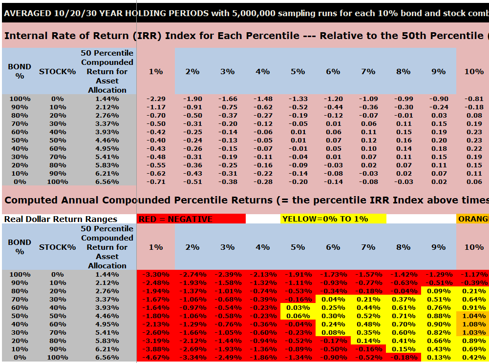
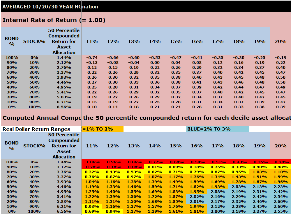
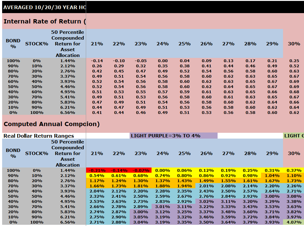
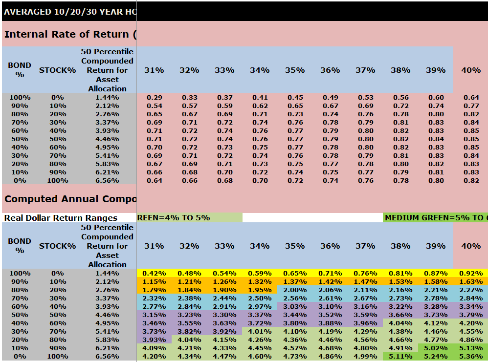
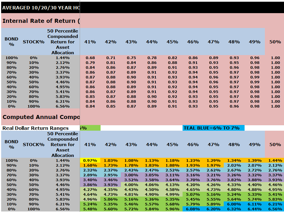
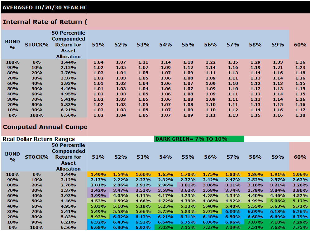
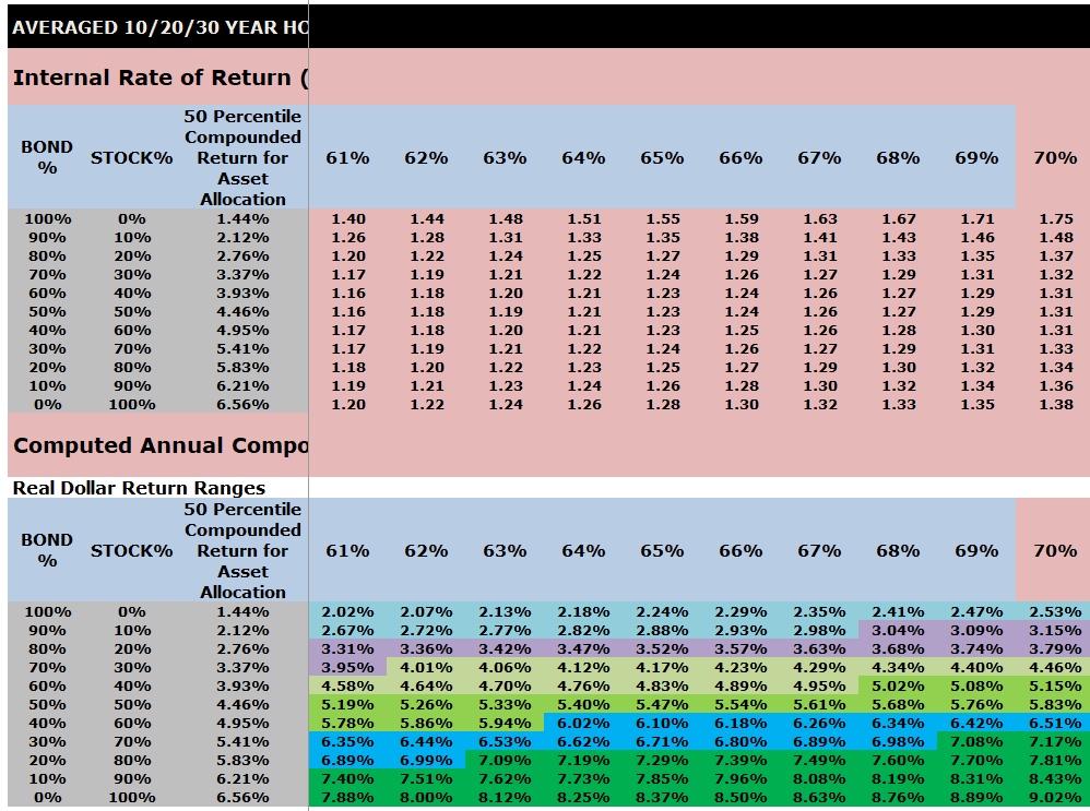
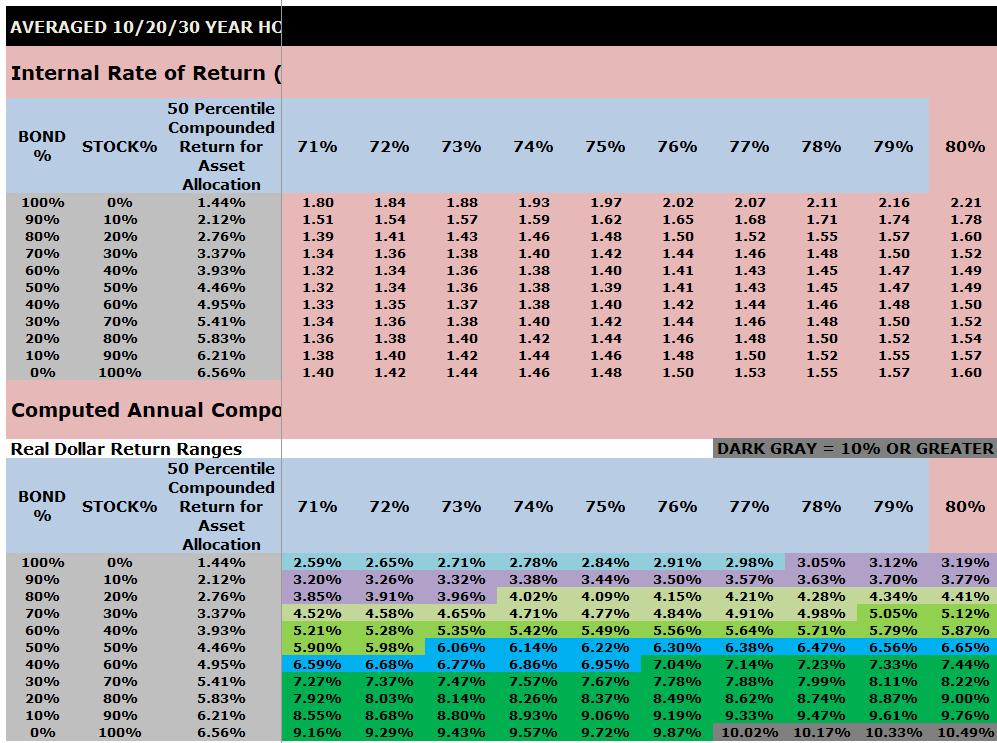
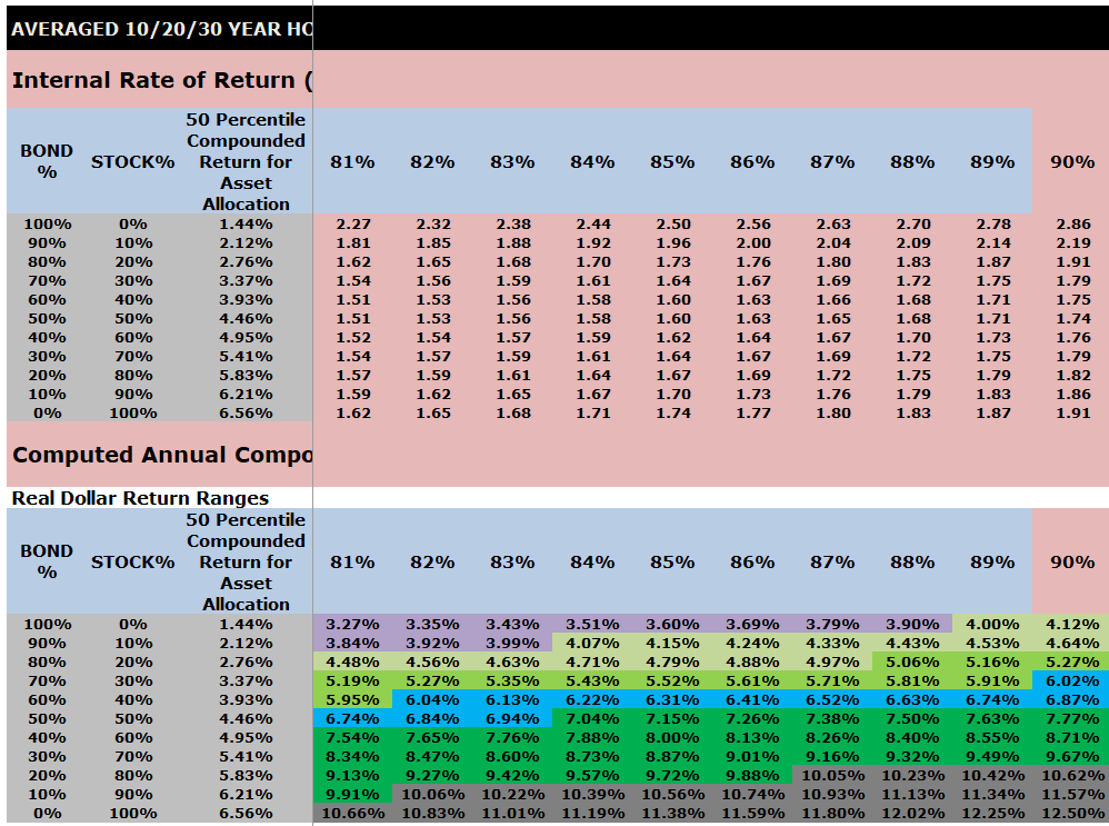
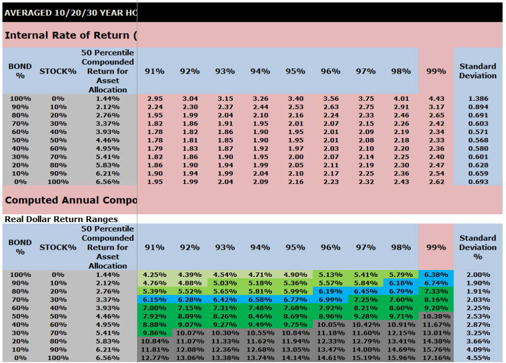
Averaged 10/20/30 Year IRR Index Ratios for a $1000 initial investment and $0 or $100 subsequent annual investments

The top part of this chart shows the Internal Rate of Return (IRR) index ratios by asset allocation that are embedded into VeriPlan.

The lower part of this chart shows the computed annual compounded returns for the 1928 through 2023 study period. Performance percentiles are segregated by color to make the chart more easy to understand.

Note that the output tables below from VeriPlan’s Excel Monte Carlo analysis study of investment risk and return are very wide and require horizontal scrolling. Therefore, to obtain screenshots of the entire table, it was necessary to use ten screenshots and present them in a stack below. Each of these ten screenshots has the same first three columns so that the reader can understand the decile asset allocations between stocks and bonds.

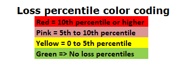
Color coding of compounded annual, US historical real dollar (with inflation removed) investment returns in the charts below:

Note: If you were using VeriPlan, you would scroll horizontally to see all the percentiles in the screenshots below >>>>>

INSERT SCREEN SHOTS OF AVERAGES

Summary notes:

A) Bonds = US 10-Year Treasury Bonds cumulative annual (geometric) total return with interest (01/01/1928 to 12/31/2023 = 96 years)

B) Stocks = US S&P Index cumulative annual (geometric) total return with dividends (01/01/1928 to 12/31/2023 = 96 years)

C) Inflation = US Consumer Price Index (CPI-U) (01/01/1928 to 12/31/2023 = 96 years)

D) Annual inflation was removed from bond and stock annual percentage returns to derive real, constant purchasing power dollar percentage returns

E) An annual Bond and Stock weighted average real dollar return was derived for each year from 1928 to 2023 for each decile asset allocation portfolio.

F) 5,000,000 Monte Carlo statistical sampling runs were done for each combination of the a) 11 bond/stock decile portfolios, b) 6 holding periods (10, 20, 30, 40, 50, & 60 years), and c) 2 investment models ($1,000 initial and either $0 or $100 each year thereafter)

G) The ending portfolio values of each outcome within each 5,000,000 sampling run were sorted from the least to greatest. Then single percentiles from 1% to 99% were calculated. Each single percentile represented 50,000 outcomes. H) For each of the statistical sampling runs, the Internal Rate of Return (IRR) was calculated to derive a distribution index with the 50% value set to 1 (one).

I) Charts were developed for percentage portfolio returns across the 11 portfolios and percentile from 1% to 99% for each of the six holding periods and two investment models.

J) Charts were color-coded with the standard method shown above, so that they could be visually evaluated and compared more easily.

K) This evaluation determined that the two investment models and 10, 20, and 30 year holding periods were sufficiently similar to be blended and used aa a single distribution model for evaluating the variability of lifetime projections. Note that the 40, 50, and 60 year periods were similar to the 30 year period with mildly reduced variation.

L) Among the 10, 20, and 30 year periods, the 10 year period demonstrated the most variability and the 30 period the least. Nevertheless, a focus on the higher variability of shorter-periods can distort decision-making about multi-decade portfolio management strategies. Thus, it was decided blend the three periods into a single aggregate.

M) The 40, 50, and 50 year periods were not included, because they were increasingly similar and would tend to obscure the higher variability of the blended 10, 20, and 30 year periods.